Introduction
Blueprinty is a small firm that makes software for developing blueprints specifically for submitting patent applications to the US patent office. Their marketing team would like to make the claim that patent applicants using Blueprinty’s software are more successful in getting their patent applications approved. Ideal data to study such an effect might include the success rate of patent applications before using Blueprinty’s software and after using it. Unfortunately, such data is not available.
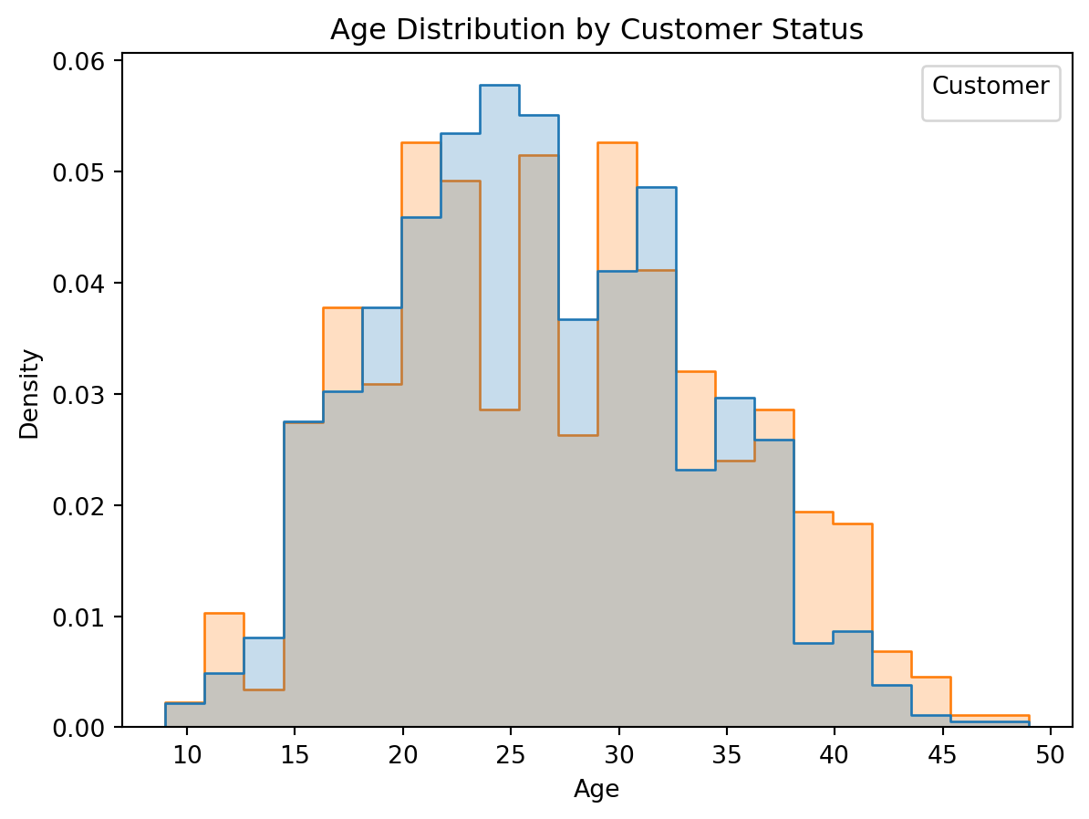
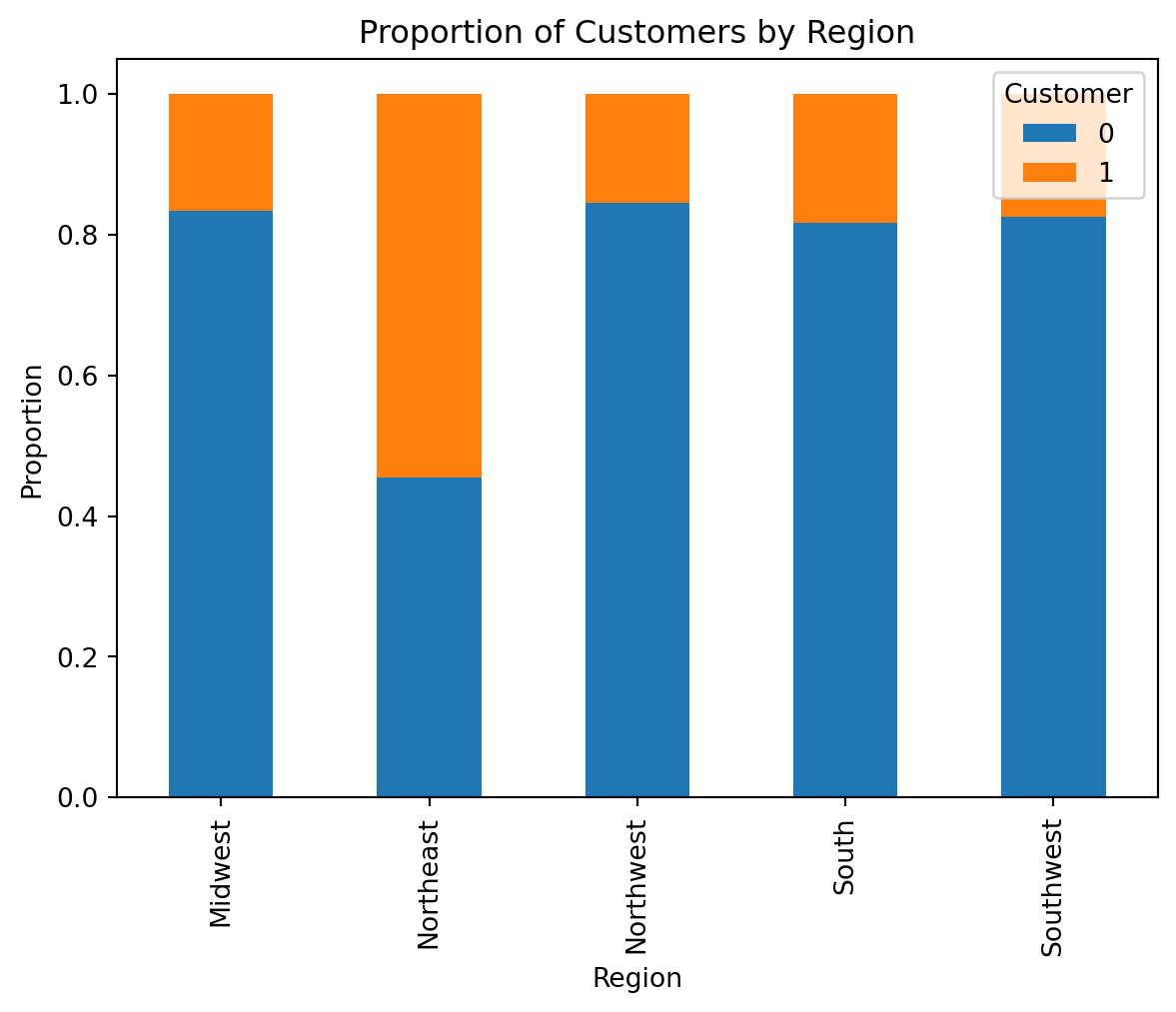
However, Blueprinty has collected data on 1,500 mature (non-startup) engineering firms. The data include each firm’s number of patents awarded over the last 5 years, regional location, age since incorporation, and whether or not the firm uses Blueprinty’s software. The marketing team would like to use this data to make the claim that firms using Blueprinty’s software are more successful in getting their patent applications approved.
Estimation of Simple Poisson Model
Since our outcome variable of interest can only be small integer values per a set unit of time, we can use a Poisson density to model the number of patents awarded to each engineering firm over the last 5 years. We start by estimating a simple Poisson model via Maximum Likelihood.
Let ( Y_1, Y_2, , Y_n () ). The probability mass function is:
[ f(Y_i ) = ]
Then the likelihood function for a sample of size ( n ) is:
[ (Y_1, , Y_n) = _{i=1}^{n} ]
Taking the natural logarithm to get the log-likelihood:
[ () = _{i=1}^{n} ( -+ Y_i - Y_i! ) ]
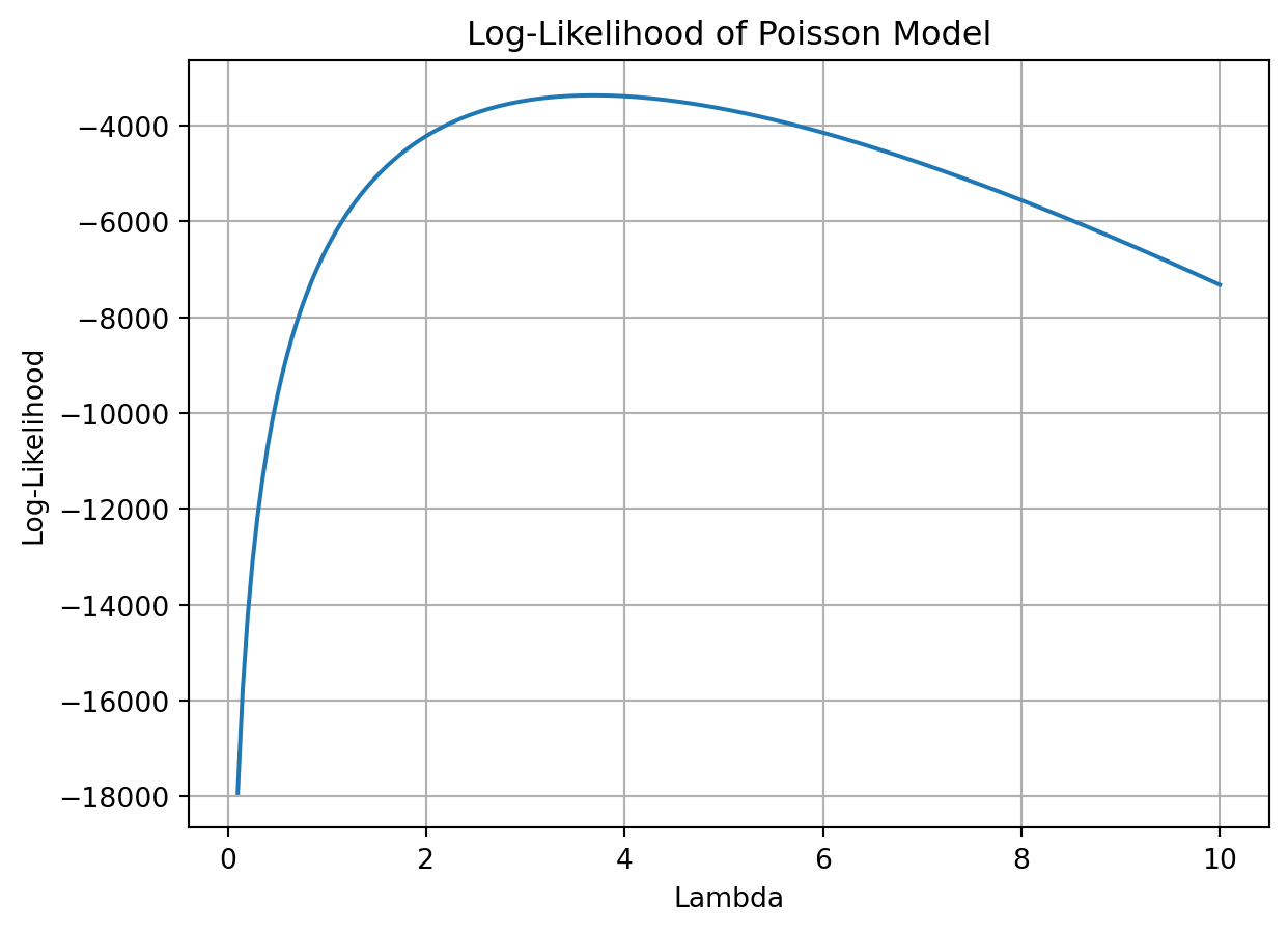
This is the log-likelihood expression we will use to estimate ( ) in our simple Poisson model.
The log-likelihood curve reaches a clear peak, suggesting the maximum likelihood estimate (MLE) of ( ) lies around that peak.
This visual check helps confirm the function is well-behaved and the model is appropriate for estimating a central rate parameter from count data.
We start with the log-likelihood for ( n ) i.i.d. observations from a Poisson distribution:
[ () = _{i=1}^{n} ( -+ Y_i - Y_i! ) ]
To find the MLE of ( ), we take the first derivative with respect to ( ):
[ = {i=1}^{n} ( -1 + ) = -n + {i=1}^{n} Y_i ]
Set the derivative equal to zero and solve for ( ):
[ -n + {i=1}^{n} Y_i = 0 {i=1}^{n} Y_i = n = _{i=1}^{n} Y_i = {Y} ]
Thus, the MLE of ( ) is simply the sample mean ( {Y} ).
This makes intuitive sense, since the Poisson distribution has both its mean and variance equal to ( ).
MLE of lambda (numerical optimization): 3.6847
Sample mean of Y: 3.6847
Using numerical optimization, the estimated MLE of ( ) is approximately {lambda_mle:.4f},
which aligns closely with the sample mean ( {Y} = {sample_mean:.4f} ).
This matches our earlier mathematical derivation, confirming that the Poisson MLE for ( ) is the mean of the observed data.
Estimation of Poisson Regression Model
Next, we extend our simple Poisson model to a Poisson Regression Model such that \(Y_i = \text{Poisson}(\lambda_i)\) where \(\lambda_i = \exp(X_i'\beta)\). The interpretation is that the success rate of patent awards is not constant across all firms (\(\lambda\)) but rather is a function of firm characteristics \(X_i\). Specifically, we will use the covariates age, age squared, region, and whether the firm is a customer of Blueprinty.
todo: Use your function along with R’s optim() or Python’s sp.optimize() to find the MLE vector and the Hessian of the Poisson model with covariates. Specifically, the first column of X should be all 1’s to enable a constant term in the model, and the subsequent columns should be age, age squared, binary variables for all but one of the regions, and the binary customer variable. Use the Hessian to find standard errors of the beta parameter estimates and present a table of coefficients and standard errors.
         Current function value: 3258.072145
         Iterations: 18
         Function evaluations: 252
         Gradient evaluations: 28
| 0 |
intercept |
1.3447 |
0.0344 |
| 1 |
age_std |
-0.0577 |
0.0149 |
| 2 |
age_sq_std |
-0.1558 |
0.0172 |
| 3 |
iscustomer |
0.2076 |
0.0314 |
| 4 |
Northeast |
0.0292 |
0.0382 |
| 5 |
Northwest |
-0.0176 |
0.0231 |
| 6 |
South |
0.0566 |
0.0452 |
| 7 |
Southwest |
0.0506 |
0.0417 |
The coefficients represent the estimated effect of each variable on the log expected patent count.
- Being a customer of Blueprinty is associated with a significant increase in patent counts (β = 0.208, SE = 0.031).
- Age has a small negative effect, and the negative age-squared term suggests a concave relationship — i.e., patenting peaks in mid-career.
- Regional effects are relatively minor, with South and Southwest showing small positive deviations.
                 Generalized Linear Model Regression Results
==============================================================================
Dep. Variable:                      y   No. Observations:                 1500
Model:                            GLM   Df Residuals:                     1492
Model Family:                 Poisson   Df Model:                            7
Link Function:                    Log   Scale:                          1.0000
Method:                          IRLS   Log-Likelihood:                -3258.1
Date:                Tue, 06 Jan 2026   Deviance:                       2143.3
Time:                        21:15:39   Pearson chi2:                 2.07e+03
No. Iterations:                     5   Pseudo R-squ. (CS):             0.1360
Covariance Type:            nonrobust
==============================================================================
                 coef    std err          z      P>|z|      [0.025      0.975]
------------------------------------------------------------------------------
const          1.3447      0.038     35.059      0.000       1.270       1.420
x1            -0.0577      0.015     -3.843      0.000      -0.087      -0.028
x2            -0.1558      0.014    -11.513      0.000      -0.182      -0.129
x3             0.2076      0.031      6.719      0.000       0.147       0.268
x4             0.0292      0.044      0.669      0.504      -0.056       0.115
x5            -0.0176      0.054     -0.327      0.744      -0.123       0.088
x6             0.0566      0.053      1.074      0.283      -0.047       0.160
x7             0.0506      0.047      1.072      0.284      -0.042       0.143
==============================================================================
To confirm the accuracy of our custom maximum likelihood estimation (MLE), we refit the same Poisson regression using Python’s built-in statsmodels.GLM() function.
The resulting coefficients and standard errors were nearly identical to our hand-coded implementation, validating both the numerical optimization and our understanding of Poisson regression mechanics.
Average increase in predicted patents from being a customer: 0.7928
To assess the effect of Blueprinty’s software on patent success, we simulated expected patent counts for all firms under two scenarios:
one where no firms were customers, and another where all firms were.
The analysis reveals that, on average, being a Blueprinty customer increases expected patent output by approximately 0.79 patents per firm.
This suggests a meaningful positive effect of the software on innovation activity.
AirBnB Case Study
Introduction
AirBnB is a popular platform for booking short-term rentals. In March 2017, students Annika Awad, Evan Lebo, and Anna Linden scraped of 40,000 Airbnb listings from New York City. The data include the following variables:
- `id` = unique ID number for each unit
- `last_scraped` = date when information scraped
- `host_since` = date when host first listed the unit on Airbnb
- `days` = `last_scraped` - `host_since` = number of days the unit has been listed
- `room_type` = Entire home/apt., Private room, or Shared room
- `bathrooms` = number of bathrooms
- `bedrooms` = number of bedrooms
- `price` = price per night (dollars)
- `number_of_reviews` = number of reviews for the unit on Airbnb
- `review_scores_cleanliness` = a cleanliness score from reviews (1-10)
- `review_scores_location` = a "quality of location" score from reviews (1-10)
- `review_scores_value` = a "quality of value" score from reviews (1-10)
- `instant_bookable` = "t" if instantly bookable, "f" if not
| 0 |
1 |
2515 |
3130 |
4/2/2017 |
9/6/2008 |
Private room |
1.0 |
1.0 |
59 |
150 |
9.0 |
9.0 |
9.0 |
f |
| 1 |
2 |
2595 |
3127 |
4/2/2017 |
9/9/2008 |
Entire home/apt |
1.0 |
0.0 |
230 |
20 |
9.0 |
10.0 |
9.0 |
f |
| 2 |
3 |
3647 |
3050 |
4/2/2017 |
11/25/2008 |
Private room |
1.0 |
1.0 |
150 |
0 |
NaN |
NaN |
NaN |
f |
| 3 |
4 |
3831 |
3038 |
4/2/2017 |
12/7/2008 |
Entire home/apt |
1.0 |
1.0 |
89 |
116 |
9.0 |
9.0 |
9.0 |
f |
| 4 |
5 |
4611 |
3012 |
4/2/2017 |
1/2/2009 |
Private room |
NaN |
1.0 |
39 |
93 |
9.0 |
8.0 |
9.0 |
t |
Unnamed: 0                       0
id                               0
days                             0
last_scraped                     0
host_since                      35
room_type                        0
bathrooms                      160
bedrooms                        76
price                            0
number_of_reviews                0
review_scores_cleanliness    10195
review_scores_location       10254
review_scores_value          10256
instant_bookable                 0
dtype: int64
                 Generalized Linear Model Regression Results
==============================================================================
Dep. Variable:                      y   No. Observations:                30160
Model:                            GLM   Df Residuals:                    30149
Model Family:                 Poisson   Df Model:                           10
Link Function:                    Log   Scale:                          1.0000
Method:                          IRLS   Log-Likelihood:            -5.2418e+05
Date:                Tue, 06 Jan 2026   Deviance:                   9.2689e+05
Time:                        21:15:40   Pearson chi2:                 1.37e+06
No. Iterations:                    10   Pseudo R-squ. (CS):             0.6840
Covariance Type:            nonrobust
==============================================================================
                 coef    std err          z      P>|z|      [0.025      0.975]
------------------------------------------------------------------------------
const          3.5533      0.016    219.754      0.000       3.522       3.585
x1            -0.1177      0.004    -31.394      0.000      -0.125      -0.110
x2             0.0741      0.002     37.197      0.000       0.070       0.078
x3             0.1131      0.001     75.611      0.000       0.110       0.116
x4            -0.0769      0.002    -47.796      0.000      -0.080      -0.074
x5            -0.0911      0.002    -50.490      0.000      -0.095      -0.088
x6             0.3459      0.003    119.666      0.000       0.340       0.352
x7            -0.0034      0.002     -2.151      0.031      -0.006      -0.000
x8             0.0635      0.000    129.755      0.000       0.063       0.064
x9            -0.0105      0.003     -3.847      0.000      -0.016      -0.005
x10           -0.2463      0.009    -28.578      0.000      -0.263      -0.229
==============================================================================
We modeled the number of reviews (as a proxy for bookings) using Poisson regression. Key findings include:
- Instant bookable listings are significantly more likely to get reviews — suggesting ease of booking matters to users.
- Larger listings (more bedrooms) and cleanliness scores are also strong positive predictors.
- Shared rooms have much fewer bookings than entire homes, and Private rooms also see reduced volume.
- Higher prices slightly reduce bookings, consistent with price sensitivity.
- “Value” and “location” scores were surprisingly negative, possibly reflecting underlying price or geography-related confounders.
Overall, the model helps identify which listing attributes are associated with higher demand in NYC’s Airbnb market.