Multinomial Logit Model

This assignment expores two methods for estimating the MNL model: (1) via Maximum Likelihood, and (2) via a Bayesian approach using a Metropolis-Hastings MCMC algorithm.

1. Likelihood for the Multi-nomial Logit (MNL) Model

Suppose we have \(i=1,\ldots,n\) consumers who each select exactly one product \(j\) from a set of \(J\) products. The outcome variable is the identity of the product chosen \(y_i \in \{1, \ldots, J\}\) or equivalently a vector of \(J-1\) zeros and \(1\) one, where the \(1\) indicates the selected product. For example, if the third product was chosen out of 3 products, then either \(y=3\) or \(y=(0,0,1)\) depending on how we want to represent it. Suppose also that we have a vector of data on each product \(x_j\) (eg, brand, price, etc.).

We model the consumer’s decision as the selection of the product that provides the most utility, and we’ll specify the utility function as a linear function of the product characteristics:

\[ U_{ij} = x_j'\beta + \epsilon_{ij} \]

where \(\epsilon_{ij}\) is an i.i.d. extreme value error term.

The choice of the i.i.d. extreme value error term leads to a closed-form expression for the probability that consumer \(i\) chooses product \(j\):

\[ \mathbb{P}_i(j) = \frac{e^{x_j'\beta}}{\sum_{k=1}^Je^{x_k'\beta}} \]

For example, if there are 3 products, the probability that consumer \(i\) chooses product 3 is:

\[ \mathbb{P}_i(3) = \frac{e^{x_3'\beta}}{e^{x_1'\beta} + e^{x_2'\beta} + e^{x_3'\beta}} \]

A clever way to write the individual likelihood function for consumer \(i\) is the product of the \(J\) probabilities, each raised to the power of an indicator variable (\(\delta_{ij}\)) that indicates the chosen product:

\[ L_i(\beta) = \prod_{j=1}^J \mathbb{P}_i(j)^{\delta_{ij}} = \mathbb{P}_i(1)^{\delta_{i1}} \times \ldots \times \mathbb{P}_i(J)^{\delta_{iJ}}\]

Notice that if the consumer selected product \(j=3\), then \(\delta_{i3}=1\) while \(\delta_{i1}=\delta_{i2}=0\) and the likelihood is:

\[ L_i(\beta) = \mathbb{P}_i(1)^0 \times \mathbb{P}_i(2)^0 \times \mathbb{P}_i(3)^1 = \mathbb{P}_i(3) = \frac{e^{x_3'\beta}}{\sum_{k=1}^3e^{x_k'\beta}} \]

The joint likelihood (across all consumers) is the product of the \(n\) individual likelihoods:

\[ L_n(\beta) = \prod_{i=1}^n L_i(\beta) = \prod_{i=1}^n \prod_{j=1}^J \mathbb{P}_i(j)^{\delta_{ij}} \]

And the joint log-likelihood function is:

\[ \ell_n(\beta) = \sum_{i=1}^n \sum_{j=1}^J \delta_{ij} \log(\mathbb{P}_i(j)) \]

2. Simulate Conjoint Data

We will simulate data from a conjoint experiment about video content streaming services. We elect to simulate 100 respondents, each completing 10 choice tasks, where they choose from three alternatives per task. For simplicity, there is not a “no choice” option; each simulated respondent must select one of the 3 alternatives.

Each alternative is a hypothetical streaming offer consistent of three attributes: (1) brand is either Netflix, Amazon Prime, or Hulu; (2) ads can either be part of the experience, or it can be ad-free, and (3) price per month ranges from $4 to $32 in increments of $4.

The part-worths (ie, preference weights or beta parameters) for the attribute levels will be 1.0 for Netflix, 0.5 for Amazon Prime (with 0 for Hulu as the reference brand); -0.8 for included adverstisements (0 for ad-free); and -0.1*price so that utility to consumer \(i\) for hypothethical streaming service \(j\) is

\[ u_{ij} = (1 \times Netflix_j) + (0.5 \times Prime_j) + (-0.8*Ads_j) - 0.1\times Price_j + \varepsilon_{ij} \]

where the variables are binary indicators and \(\varepsilon\) is Type 1 Extreme Value (ie, Gumble) distributed.

The following code provides the simulation of the conjoint data.

import pandas as pd
import numpy as np

# Set seed for reproducibility
np.random.seed(123)

# Define attributes
brands = ["N", "P", "H"]  # Netflix, Prime, Hulu
ads = ["Yes", "No"]
prices = np.arange(8, 33, 4)

# Generate all possible profiles
profiles = pd.DataFrame([(b, a, p) for b in brands for a in ads for p in prices],
                        columns=["brand", "ad", "price"])

# Utility functions
b_util = {"N": 1.0, "P": 0.5, "H": 0.0}
a_util = {"Yes": -0.8, "No": 0.0}
p_util = lambda p: -0.1 * p

# Simulation parameters
n_peeps = 100
n_tasks = 10
n_alts = 3

# Simulate one respondent
def sim_one(id):
    datlist = []
    for t in range(1, n_tasks + 1):
        sampled = profiles.sample(n=n_alts, replace=False).copy()
        sampled.insert(0, "task", t)
        sampled.insert(0, "resp", id)
        sampled["v"] = (
            sampled["brand"].map(b_util) +
            sampled["ad"].map(a_util) +
            p_util(sampled["price"])
        ).round(10)
        sampled["e"] = -np.log(-np.log(np.random.rand(n_alts)))
        sampled["u"] = sampled["v"] + sampled["e"]
        sampled["choice"] = (sampled["u"] == sampled["u"].max()).astype(int)
        datlist.append(sampled)
    return pd.concat(datlist, ignore_index=True)

# Generate data
conjoint_data = pd.concat([sim_one(i) for i in range(1, n_peeps + 1)], ignore_index=True)

# Keep only observable variables
conjoint_data = conjoint_data[["resp", "task", "brand", "ad", "price", "choice"]]

3. Preparing the Data for Estimation

The “hard part” of the MNL likelihood function is organizing the data, as we need to keep track of 3 dimensions (consumer \(i\), covariate \(k\), and product \(j\)) instead of the typical 2 dimensions for cross-sectional regression models (consumer \(i\) and covariate \(k\)). The fact that each task for each respondent has the same number of alternatives (3) helps. In addition, we need to convert the categorical variables for brand and ads into binary variables.

To prepare the data: - We created dummy variables for the brand attribute. Specifically, we included binary indicators for Netflix and Prime Video, using Hulu as the baseline. - The ad feature was converted into a binary variable, where 1 indicates the presence of ads and 0 indicates an ad-free option. - We retained the price and choice columns in their original form.

Below is the Python code used for data preprocessing. The previewed table shows that each row corresponds to one product alternative shown in a choice task.

import pandas as pd

# Loading and and preprocessing of  data
df = pd.read_csv('conjoint_data.csv')
df = pd.get_dummies(df, columns=["brand"], drop_first=True)
df["ad"] = df["ad"].map({"Yes": 1, "No": 0})
df.rename(columns={"brand_N": "netflix", "brand_P": "prime"}, inplace=True)
df.head()

# Create design matrix and response vector

X_columns = ["netflix", "prime", "ad", "price"]
X = df[X_columns].values
y = df["choice"].values
df["choice_set"] = df["resp"].astype(str) + "_" + df["task"].astype(str)
choice_sets = df["choice_set"].values

4. Estimation via Maximum Likelihood

We begin by defining the log-likelihood function for the Multinomial Logit (MNL) model. For each choice set (i.e., a group of three product alternatives shown to a respondent), we compute the probability of the selected alternative using the softmax function applied to the utility values. These utilities are linear combinations of the feature values and coefficients (betas).

The function below returns the negative log-likelihood, which we will minimize using scipy.optimize.

def log_likelihood(beta, X, y, groups):
    df_ll = pd.DataFrame(X, columns=["netflix", "prime", "ad", "price"]).copy()
    df_ll["choice"] = y
    df_ll["group"] = groups

    # Compute deterministic utility
    df_ll["utility"] = df_ll[["netflix", "prime", "ad", "price"]].dot(beta)

    # Group-wise max utility for numerical stability
    df_ll["max_util"] = df_ll.groupby("group")["utility"].transform("max")

    # Ensure numeric type before exponentiation
    diff = np.asarray(df_ll["utility"] - df_ll["max_util"], dtype=np.float64)
    df_ll["exp_util"] = np.exp(diff)

    # Denominator: sum of exponentiated utilities within each group
    df_ll["sum_exp_util"] = df_ll.groupby("group")["exp_util"].transform("sum")

    # Compute probabilities
    df_ll["prob"] = df_ll["exp_util"] / df_ll["sum_exp_util"]

    # Log-likelihood of chosen alternatives
    log_probs = np.log(df_ll.loc[df_ll["choice"] == 1, "prob"])

    return -log_probs.sum()

To estimate the parameters of the multinomial logit (MNL) model efficiently, we implemented a vectorized version of the log-likelihood function using pandas and NumPy. This function calculates the probability of each chosen alternative within a choice task using the softmax transformation of the deterministic utility.

Rather than iterating over each individual choice task in Python loops (which becomes computationally expensive for larger datasets or when running MCMC sampling), we use groupby().transform() to: - Calculate utilities for all alternatives - Normalize them within each choice task - Compute the probabilities and log-likelihood in a fully vectorized way

This approach significantly reduces computation time while still maintaining transparency and fidelity to the underlying MNL structure. It’s especially important when running thousands of iterations in Metropolis-Hastings sampling, where performance bottlenecks can severely impact feasibility.

from scipy.optimize import minimize
import numpy as np

# Start with zero coefficients
initial_beta = np.zeros(X.shape[1])

# Minimize the negative log-likelihood
result = minimize(
    log_likelihood,
    initial_beta,
    args=(X, y, choice_sets),
    method="BFGS",
    options={"disp": True}
)

# Estimated coefficients
beta_hat = result.x

# Standard errors from inverse Hessian
hessian_inv = result.hess_inv
se = np.sqrt(np.diag(hessian_inv))

# 95% confidence intervals
z = 1.96
conf_int = np.array([beta_hat - z * se, beta_hat + z * se]).T

# Combining everything into a table
import pandas as pd
summary_df = pd.DataFrame({
    "Estimate": beta_hat,
    "Std. Error": se,
    "95% CI Lower": conf_int[:, 0],
    "95% CI Upper": conf_int[:, 1]
}, index=["netflix", "prime", "ad", "price"])

Optimization terminated successfully.
         Current function value: 879.855368
         Iterations: 12
         Function evaluations: 85
         Gradient evaluations: 17

We estimated the parameters of the multinomial logit model using the BFGS algorithm via scipy.optimize.minimize(), minimizing the negative log-likelihood function defined earlier. The model includes binary indicators for netflix, prime, and ad, with hulu and no ads as the respective baseline categories, along with the continuous variable price.

The table below summarizes the parameter estimates, standard errors (from the inverse Hessian), and 95% confidence intervals:

summary_df.round(3)

	Estimate	Std. Error	95% CI Lower	95% CI Upper
netflix	0.941	0.114	0.718	1.164
prime	0.502	0.121	0.265	0.739
ad	-0.732	0.088	-0.905	-0.559
price	-0.099	0.006	-0.112	-0.087

Interpreting the Estimates

• Brand Preference: Netflix and Prime are both preferred over the baseline (Hulu), with Netflix receiving the highest utility.

• Ad Dislike: The negative coefficient for ad confirms that respondents significantly prefer ad-free experiences.

• Price Sensitivity: The negative and significant coefficient for price aligns with economic intuition — as price increases, utility decreases.

5. Estimation via Bayesian Methods

import numpy as np

# Log-prior function
def log_prior(beta):
    # Priors: N(0,5) for all except price (N(0,1))
    prior = -0.5 * ((beta[0]/np.sqrt(5))**2 +
                    (beta[1]/np.sqrt(5))**2 +
                    (beta[2]/np.sqrt(5))**2 +
                    (beta[3]/1)**2)
    return prior

# Log-posterior function
def log_posterior(beta, X, y, groups):
    return -log_likelihood(beta, X, y, groups) + log_prior(beta)

# MCMC settings
n_steps = 11000
burn_in = 1000
n_params = X.shape[1]

# Proposal distribution: diagonal covariances
proposal_sds = [0.05, 0.05, 0.05, 0.005]

# Storage
samples = np.zeros((n_steps, n_params))
beta_current = np.zeros(n_params)
log_post_current = log_posterior(beta_current, X, y, choice_sets)

# Metropolis-Hastings loop
for step in range(n_steps):
    # Propose new beta from independent normal perturbations
    beta_proposal = beta_current + np.random.normal(0, proposal_sds)

    # Compute log-posterior
    log_post_proposal = log_posterior(beta_proposal, X, y, choice_sets)

    # Acceptance probability
    accept_prob = min(1, np.exp(log_post_proposal - log_post_current))

    # Accept or reject
    if np.random.rand() < accept_prob:
        beta_current = beta_proposal
        log_post_current = log_post_proposal

    samples[step] = beta_current

import numpy as np
import pandas as pd

# Assume 'samples' is your MCMC output from earlier
# Retain only the last 10,000 samples (after 1,000 burn-in)
posterior_samples = samples[1000:]

# Posterior summaries
posterior_means = posterior_samples.mean(axis=0)
posterior_stds = posterior_samples.std(axis=0)
z = 1.96
posterior_ci = np.array([
    posterior_means - z * posterior_stds,
    posterior_means + z * posterior_stds
]).T

# Create summary table
posterior_summary = pd.DataFrame({
    "Posterior Mean": posterior_means,
    "Posterior SD": posterior_stds,
    "95% CI Lower": posterior_ci[:, 0],
    "95% CI Upper": posterior_ci[:, 1]
}, index=["netflix", "prime", "ad", "price"])

posterior_summary.round(3)

	Posterior Mean	Posterior SD	95% CI Lower	95% CI Upper
netflix	0.934	0.106	0.726	1.141
prime	0.490	0.108	0.279	0.702
ad	-0.726	0.089	-0.901	-0.552
price	-0.100	0.006	-0.112	-0.087

Posterior Distribution Interpretations

The table above presents the posterior summaries based on 10,000 samples from the Metropolis-Hastings sampler (after a burn-in of 1,000 iterations). The posterior means are highly consistent with the Maximum Likelihood Estimates, which confirms the stability of the model.

• Brand Preferences:
  • Consumers prefer Netflix the most (\(\beta = 0.934\)), followed by Prime (\(\beta = 0.49\)), both relative to Hulu (the omitted baseline).
  • The credible intervals for both exclude zero, reinforcing their significance.
• Ad Aversion:
  • The negative coefficient on ad (\(\beta = -0.726\)) confirms a strong aversion to advertisements.
• Price Sensitivity:
  • As expected, the coefficient for price is negative (\(\beta = -0.1\)), with a narrow 95% credible interval, showing consistent consumer price sensitivity across the sample.

Overall, the Bayesian results closely align with those from the frequentist estimation, increasing confidence in the model’s conclusions. The slight broadening of credible intervals compared to confidence intervals is expected due to the incorporation of prior uncertainty.

import matplotlib.pyplot as plt

# Plot for β_price (index = 3)
fig, axs = plt.subplots(2, 1, figsize=(10, 6))

axs[0].plot(posterior_samples[:, 3])
axs[0].set_title("Trace Plot for β_price")
axs[0].set_xlabel("Iteration")
axs[0].set_ylabel("Value")

axs[1].hist(posterior_samples[:, 3], bins=30, density=True)
axs[1].set_title("Posterior Distribution for β_price")
axs[1].set_xlabel("β_price")
axs[1].set_ylabel("Density")

plt.tight_layout()
plt.show()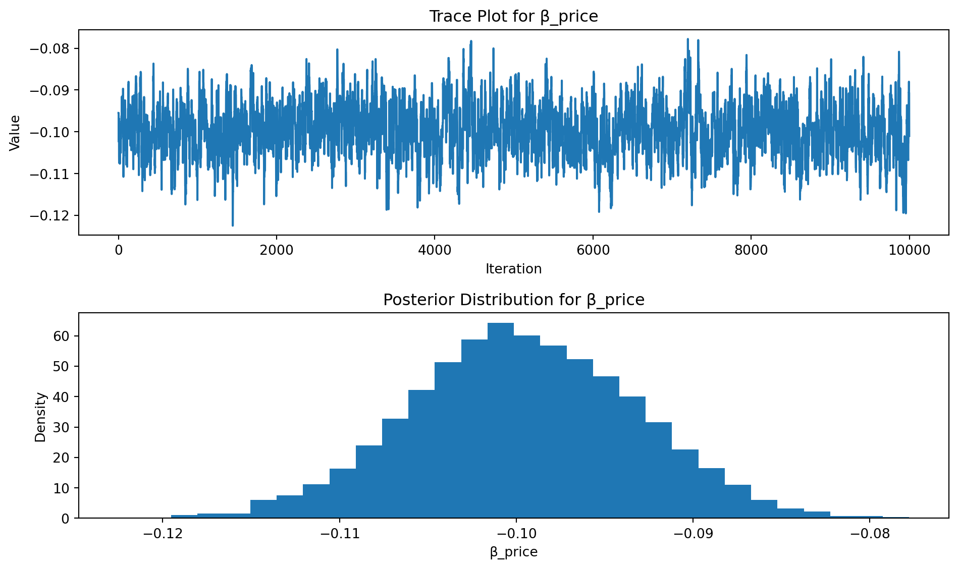

Plot Interpretation

The trace plot and posterior distribution of \(\beta_{\text{price}}\) illustrate stable and well-behaved sampling from the posterior.

• The trace plot shows excellent mixing across all 10,000 retained samples, with no apparent drift, burn-in artifacts, or convergence issues. This is a strong indication that the Markov chain is sampling effectively from the target posterior distribution.

• The posterior histogram is bell-shaped and centered tightly around -0.10, with most mass falling between -0.112 and -0.08. This reflects precise and confident estimation of consumers’ price sensitivity: as price increases, utility reliably decreases.

Together, these plots confirm that the MCMC chain for \(\beta_{\text{price}}\) has converged and sampled efficiently, making the resulting posterior summary highly trustworthy.

6. Discussion

Had we not simulated the data ourselves, we would still be able to draw clear and interpretable insights from the estimated parameters. The results from both the MLE and Bayesian methods are consistent and reinforce meaningful patterns in consumer preference:

• The fact that \(\beta_{\text{Netflix}} > \beta_{\text{Prime}}\) suggests that consumers prefer Netflix over Prime Video, all else equal. Since Hulu is the baseline, both brands are more desirable, but Netflix provides the highest utility on average.
• The consistently negative value of \(\beta_{\text{price}}\), with tight credible intervals (e.g., [−0.112, −0.08]), confirms that price negatively influences utility — a core principle in consumer choice modeling.

These results align with economic intuition and show up robustly across both frequentist and Bayesian approaches. The credible intervals in the Bayesian framework also provide a probabilistic interpretation of uncertainty, enhancing the confidence in our conclusions.

Moving Toward Real-World Conjoint Models

In practice, consumer preferences are rarely fixed across individuals. The standard MNL model assumes a single set of utility weights shared by everyone, which oversimplifies real-world heterogeneity. To model this variation, we would extend our framework to a:

• Multi-level model (also known as a random-parameter or hierarchical Bayes model)

In such models: - Each individual is assumed to have their own \(\beta\) coefficients, drawn from a population-level distribution (e.g., \(\beta_i \sim \mathcal{N}(\mu, \Sigma)\)). - The goal becomes estimating both the individual-level preferences and the distribution of preferences across the population.

These models are more computationally intensive, but they provide a richer, more realistic view of consumer behavior. They’re especially useful for personalized marketing, targeting, and advanced segmentation.